A gentle introduction to temporal response functions (TRFs)

This tutorial builds a TRF analysis from scratch using simulated data. The goal is to make the shape of every object explicit:

1. create stimulus features and an EEG-like response;

2. fit and inspect a TRF;

3. choose regularisation with cross-validation;

4. use banded ridge when features have different scales or reliability; and

5. encourage smooth temporal filters with quadratic regularisation.

All figures are made in notebook cells, so they are included automatically in the HTML documentation.

import time
import numpy as np
import matplotlib.pyplot as plt

from pyeeg import TRFEstimator
from pyeeg.simulate import (
    dummy_trf_kernel,
    simulate_pulse_inputs,
    simulate_smooth_input,
    simulate_trf_output,
)

plt.rcParams['figure.figsize'] = (10, 3)
plt.rcParams['figure.dpi'] = 110

/opt/hostedtoolcache/Python/3.12.14/x64/lib/python3.12/site-packages/tqdm/auto.py:21: TqdmWarning: IProgress not found. Please update jupyter and ipywidgets. See https://ipywidgets.readthedocs.io/en/stable/user_install.html
  from .autonotebook import tqdm as notebook_tqdm

1. Simulate two stimulus features

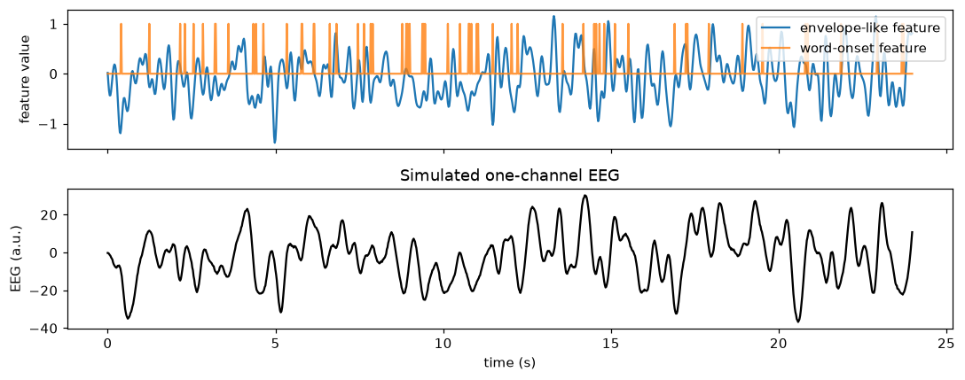
A TRF maps a time-varying feature matrix X to an EEG matrix y. Here the first feature is a smooth, envelope-like signal and the second is a sparse word-onset-like signal. We use one known kernel for each feature, then add noise.

rng = np.random.default_rng(7)
fs, duration = 50, 24
t, envelope = simulate_smooth_input(duration, fs, fmax=5, seed=7)
_, words = simulate_pulse_inputs(n_events=60, dur=duration, srate=fs, seed=8)
X = np.column_stack([envelope, words])

t_kernel, kernel = dummy_trf_kernel(-0.2, 0.6, fs, tloc=0.18, sigma=0.09)
y = (
    simulate_trf_output(t_kernel, 1.0 * kernel, envelope, fs)
    + simulate_trf_output(t_kernel, 0.7 * kernel, words, fs)
    + 0.25 * rng.standard_normal(len(t))
)[:, None]

fig, axes = plt.subplots(2, 1, sharex=True, figsize=(10, 4))
axes[0].plot(t, envelope, label='envelope-like feature')
axes[0].plot(t, words, label='word-onset feature', alpha=.8)
axes[0].legend(loc='upper right')
axes[0].set_ylabel('feature value')
axes[1].plot(t, y[:, 0], color='black')
axes[1].set(xlabel='time (s)', ylabel='EEG (a.u.)', title='Simulated one-channel EEG')
fig.tight_layout()

2. Fit the simplest TRF

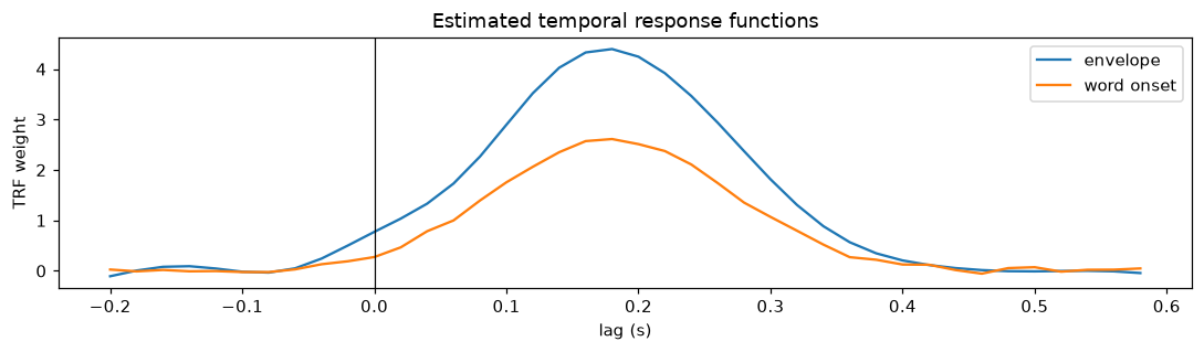
tmin and tmax define the lags (in seconds) at which the response is estimated. coef_ has shape (n_lags, n_features, n_channels).

trf = TRFEstimator(tmin=-0.2, tmax=0.6, srate=fs, alpha=10, verbose=False)
trf.fit(X, y, feat_names=['envelope', 'word onset'])
print('X:', X.shape, 'y:', y.shape, 'coef_:', trf.coef_.shape)
print(f'train correlation: {trf.score(X, y, reduce_multi="mean"):.2f}')

fig, ax = plt.subplots()
for feature, name in enumerate(trf.feat_names_):
    ax.plot(trf.times, trf.coef_[:, feature, 0], label=name)
ax.axvline(0, color='black', lw=.8)
ax.set(xlabel='lag (s)', ylabel='TRF weight', title='Estimated temporal response functions')
ax.legend()
fig.tight_layout()

X: (1200, 2) y: (1200, 1) coef_: (40, 2, 1)
train correlation: 1.00

3. Regularisation and cross-validation

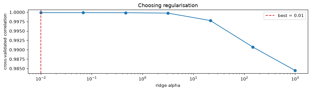
A larger ridge alpha shrinks coefficients and is useful when the lagged design matrix is noisy or collinear. Pass several values and call xfit to select the value with the best held-out correlation.

alphas = np.logspace(-2, 3, 7)
cv_trf = TRFEstimator(tmin=-0.2, tmax=0.6, srate=fs, alpha=alphas, verbose=False)
scores, best_alpha = cv_trf.xfit(X, y, n_splits=4, plot=False)
mean_scores = scores.mean(axis=(0, 1, 3))
print('best alpha:', best_alpha)

fig, ax = plt.subplots()
ax.semilogx(alphas, mean_scores, 'o-')
ax.axvline(best_alpha, color='tab:red', ls='--', label=f'best = {best_alpha:g}')
ax.set(xlabel='ridge alpha', ylabel='cross-validated correlation', title='Choosing regularisation')
ax.legend()
fig.tight_layout()

best alpha: 0.01

4. Banded ridge: one penalty per feature

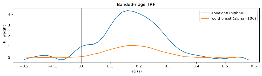
Envelope and word-level features need not deserve the same penalty. feature_alphas supplies one ridge strength per input column. The next fit deliberately penalises the sparse word feature more strongly.

banded = TRFEstimator(
    tmin=-0.2, tmax=0.6, srate=fs,
    feature_alphas=[1, 100], verbose=False,
)
banded.fit(X, y, feat_names=['envelope', 'word onset'])

fig, ax = plt.subplots()
for feature, name in enumerate(banded.feat_names_):
    ax.plot(banded.times, banded.coef_[:, feature, 0], label=f'{name} (alpha={banded.feature_alphas[feature]:g})')
ax.axvline(0, color='black', lw=.8)
ax.set(xlabel='lag (s)', ylabel='TRF weight', title='Banded-ridge TRF')
ax.legend()
fig.tight_layout()

5. Smoothness regularisation

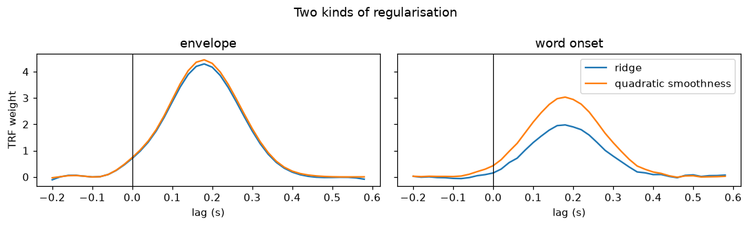
Quadratic regularisation penalises changes between neighbouring lags rather than simply shrinking every coefficient. Compare an ordinary ridge fit with quadratic_reg='smoothness'.

ridge = TRFEstimator(tmin=-0.2, tmax=0.6, srate=fs, alpha=30, verbose=False)
smooth = TRFEstimator(tmin=-0.2, tmax=0.6, srate=fs, alpha=30, quadratic_reg='smoothness', verbose=False)
ridge.fit(X, y)
smooth.fit(X, y)

fig, axes = plt.subplots(1, 2, sharey=True, figsize=(10, 3))
for feature, name in enumerate(['envelope', 'word onset']):
    axes[feature].plot(ridge.times, ridge.coef_[:, feature, 0], label='ridge')
    axes[feature].plot(smooth.times, smooth.coef_[:, feature, 0], label='quadratic smoothness')
    axes[feature].axvline(0, color='black', lw=.8)
    axes[feature].set(title=name, xlabel='lag (s)')
axes[0].set_ylabel('TRF weight')
axes[1].legend()
fig.suptitle('Two kinds of regularisation')
fig.tight_layout()

6. Timing different fitting paths

The SVD ridge path is usually the quickest choice for ordinary fits. Quadratic regularisation adds a structured matrix solve, while robust Cauchy fitting iterates several weighted fits. This small benchmark is only illustrative: timings depend on the machine and data size.

def elapsed(estimator):
    start = time.perf_counter()
    estimator.fit(X, y)
    return time.perf_counter() - start

timed = {
    'ridge (SVD)': TRFEstimator(tmin=-.2, tmax=.6, srate=fs, alpha=30, verbose=False),
    'smoothness': TRFEstimator(tmin=-.2, tmax=.6, srate=fs, alpha=30, quadratic_reg='smoothness', verbose=False),
    'robust IRLS': TRFEstimator(tmin=-.2, tmax=.6, srate=fs, loss='cauchy', robust_sigma=.25, robust_max_iter=5, verbose=False),
}
times = {name: elapsed(estimator) for name, estimator in timed.items()}
for name, seconds in times.items():
    print(f'{name:16s}: {seconds:.3f} s')

ridge (SVD)     : 0.004 s
smoothness      : 0.003 s
robust IRLS     : 0.006 s

Take-home messages

• Keep X as (samples, features) and y as (samples, channels).

• Use alpha (and cross-validation) for ordinary ridge shrinkage.

• Use feature_alphas for banded ridge when feature groups have different reliability.

• Use quadratic_reg='smoothness' when neighbouring TRF lags should vary smoothly.

• Inspect the estimated filters and held-out scores, not only the training fit.