TRF estimation: statistical inference, regularisation, and solvers

An in-depth tutorial — see A gentle introduction to TRFs for a simpler starting point.

This tutorial shows how to estimate a Temporal Response Function (TRF) with pyeeg. A TRF is a linear kernel that maps a stimulus (or any continuous predictor) onto a response:

y(t) = sum_tau h(tau) * x(t - tau) + e(t)

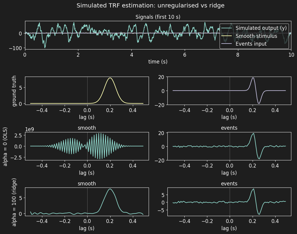
Fitting a TRF means estimating the kernel h(tau) over a window of lags [tmin, tmax] around stimulus onset. A positive lag means the response follows the stimulus: the ground-truth kernel used here peaks at +0.2 s, i.e. the response lags the stimulus by 200 ms.

What this notebook covers

1. Simulating a response driven by two predictors: a smooth continuous stimulus and an impulse-like (event) stimulus

2. Fitting TRFs with ridge regularisation — and why the smooth predictor needs it

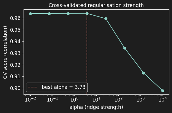
3. Selecting the regularisation strength by cross-validation (xfit)

4. Banded regularisation (feature_alphas): penalise only what needs it

5. Statistical inference: permutation test and bootstrap confidence intervals (pyeeg.stats)

6. Robust fitting (Cauchy loss) when the data contain outliers

7. Solver comparison and multi-channel TRFs

All data are simulated in-notebook (no downloads) and all randomness is seeded. A full top-to-bottom run takes a few minutes, dominated by the permutation test and the bootstrap.

import time

import numpy as np
import matplotlib.pyplot as plt

from pyeeg import TRFEstimator
from pyeeg.simulate import (
    dummy_trf_kernel,
    simulate_smooth_input,
    simulate_pulse_inputs,
    simulate_trf_output,
)
from pyeeg.stats import permutation_test_trf, bootstrap_ci_trf
from pyeeg.solvers import (
    SVDSolver,
    LSTSQSolver,
    ConjugateGradientSolver,
    IRLSSolver,
)
from pyeeg.vizu import plot_trf_signi
from pyeeg.utils import lag_matrix

# Matplotlib style (toggle dark mode here)
dark_mode = True
plt.rcParams['font.size'] = 12
plt.rcParams['axes.titlesize'] = 12
if dark_mode:
    plt.rcParams['axes.facecolor'] = '#1e1e1e'
    plt.rcParams['axes.edgecolor'] = '#ffffff'
    plt.rcParams['axes.labelcolor'] = '#ffffff'
    plt.rcParams['xtick.color'] = '#ffffff'
    plt.rcParams['ytick.color'] = '#ffffff'
    plt.rcParams['figure.facecolor'] = '#1e1e1e'
    plt.rcParams['figure.edgecolor'] = '#1e1e1e'

# Reproducibility: one seed for everything
seed = 2026
rng = np.random.default_rng(seed)  # for noise/outliers we draw ourselves

# Parameters
fs = 100  # Sampling frequency (Hz)
duration = 30  # Duration (s)
n_samples = int(fs * duration)  # Number of samples
tmin = -0.5  # Start of the TRF lag window (s)
tmax = 0.5  # End of the TRF lag window (s)
n_events = 100  # Number of events for the impulse-like stimulus
noise_rel = 0.25  # Noise std as a fraction of the clean response std

# Simulated data
# Ground-truth kernels: a Gaussian for the smooth predictor and its derivative
# (a "bipolar" kernel) for the impulse-like predictor. Both peak at +0.2 s.
t_kernel, kernel1 = dummy_trf_kernel(tmin=tmin, tmax=tmax, srate=fs,
                                     tloc=0.2, sigma=0.05, kernel_type='gaussian')
_, kernel2 = dummy_trf_kernel(tmin=tmin, tmax=tmax, srate=fs,
                              tloc=0.2, sigma=0.05, kernel_type='bipolar')
# Kernel amplitudes are arbitrary simulation choices: scale the event kernel up
# so both predictors have comparable effect sizes (otherwise the weaker feature
# is invisible to the FWE-corrected inference below)
kernel2 = 5 * kernel2

# Stimuli: one smooth continuous (low-passed noise), one impulse-like (events)
_, smooth_stimulus = simulate_smooth_input(dur=duration, srate=fs, fmax=15, seed=seed+1) # Must use different seed to not correlate noise and stim!
_, event_stimulus = simulate_pulse_inputs(n_events=n_events, dur=duration,
                                          srate=fs, seed=seed+2)

# Response: each stimulus convolved with its kernel, mixed, plus noise
y_smooth = simulate_trf_output(t_kernel, kernel1, smooth_stimulus, srate=fs)
y_event = simulate_trf_output(t_kernel, kernel2, event_stimulus, srate=fs)
y_clean = y_smooth + y_event
noise = noise_rel * y_clean.std() * rng.standard_normal(n_samples)
y = (y_clean + noise)[:, None]
noise_std = noise.std()

# Design matrix: one column per stimulus
X = np.c_[smooth_stimulus, event_stimulus]
feat_names = ['smooth', 'events']

print(f'X: {X.shape} (n_samples x n_features), y: {y.shape} (n_samples x n_channels)')
print(f'y std: {y.std():.2f} (noise std: {noise_std:.2f})')

X: (3000, 2) (n_samples x n_features), y: (3000, 1) (n_samples x n_channels)
y std: 26.37 (noise std: 6.39)

Mixing impulse-like and smooth predictors

The main issue with mixing both types of predictors is that regularisation is really only needed for the smooth continuous predictor: low-passed noise is strongly autocorrelated, so its lagged columns are nearly collinear and the unregularised fit has a huge variance. The impulse-like (event) predictor does not suffer from this.

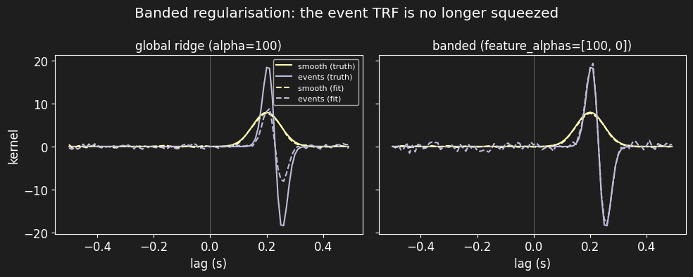
A single global ridge penalty therefore squeezes the event TRF unnecessarily. Ridge shrinks coefficient amplitude (which hurts the MSE loss), but because the shrinkage is roughly scale-uniform it barely changes the kernel shape (its correlation with the ground truth) — except for the event feature, where even the shape is slightly distorted. We can mitigate this by using banded regularisation — a separate penalty per feature (feature_alphas) — which we demonstrate below.

# First fits: construct a FRESH estimator per regularisation strength.
# (Mutating `trf.alpha` after construction is not equivalent: the estimator
# decides at construction time whether it is regularised, so a mutated
# `alpha = 0` would silently keep the ridge code path.)
with np.errstate(invalid='ignore'):
    # expected on this ill-conditioned design: the OLS covariance is
    # near-singular, so the classical SEs computed here are meaningless
    trf_ols = TRFEstimator(tmin=tmin, tmax=tmax, srate=fs, alpha=0.).fit(
        X, y, feat_names=feat_names)
trf_ridge = TRFEstimator(tmin=tmin, tmax=tmax, srate=fs, alpha=100.).fit(
    X, y, feat_names=feat_names)

print(f'OLS   (alpha=0):   max |coef| = {np.abs(trf_ols.coef_).max():.3g}  <- unstable')
print(f'ridge (alpha=100): max |coef| = {np.abs(trf_ridge.coef_).max():.3g}')

# Figure: signals, ground truth, and both fits (one panel per feature)
mosaic = [['signals', 'signals'],
          ['truth_smooth', 'truth_events'],
          ['ols_smooth', 'ols_events'],
          ['ridge_smooth', 'ridge_events']]
f, ax = plt.subplot_mosaic(mosaic, figsize=(10, 8), sharey=False)

t = np.arange(n_samples) / fs
ax['signals'].plot(t, y[:, 0], label='Simulated output (y)')
ax['signals'].plot(t, smooth_stimulus, label='Smooth stimulus')
ax['signals'].plot(t, event_stimulus, label='Events input')
ax['signals'].set_xlim(0, 10)  # first 10 s only: 3000 samples are visually dense
ax['signals'].legend(loc='upper right')
ax['signals'].set_title('Signals (first 10 s)')

ax['truth_smooth'].plot(t_kernel, kernel1, color='C1')
ax['truth_events'].plot(t_kernel, kernel2, color='C2')
trf_ols.plot(feat_id=[0, 1], ax=[ax['ols_smooth'], ax['ols_events']])
trf_ridge.plot(feat_id=[0, 1], ax=[ax['ridge_smooth'], ax['ridge_events']])

ax['signals'].set_xlabel('time (s)')
ax['truth_smooth'].set_ylabel('ground truth')
ax['ols_smooth'].set_ylabel('alpha = 0 (OLS)')
ax['ridge_smooth'].set_ylabel('alpha = 100 (ridge)')
for key, a in ax.items():
    if key != 'signals':
        a.axvline(0, color='gray', lw=0.5)
        a.set_xlabel('lag (s)')
f.suptitle('Simulated TRF estimation: unregularised vs ridge')
f.tight_layout()

OLS   (alpha=0):   max |coef| = 2.92e+09  <- unstable
ridge (alpha=100): max |coef| = 8.82

Regularisation: why, and how much?

The smooth stimulus is low-passed noise: neighbouring samples are highly correlated, so the columns of its lagged design matrix are nearly collinear. The design matrix is ill-conditioned and the ordinary least-squares solution has an enormous variance — that is why the alpha = 0 fit above blows up.

Ridge regularisation adds a penalty alpha * ||h||^2 to the loss, trading a little bias for a large variance reduction. alpha = 0 (or None) is plain OLS; a larger alpha shrinks the kernel more. Two refinements are worth knowing:

• Banded regularisation (feature_alphas): a separate penalty per feature — shown in the next section.

• Smoothness regularisation (quadratic_reg='smoothness'): penalises the roughness of the kernel (its second difference) rather than its amplitude.

How much regularisation? We can try to select alpha by cross-validation with xfit — with two honest caveats. First, xfit uses shuffled K-fold splits, which leak information across contiguous (lagged) samples. Second, and more importantly on this design: the CV score measures prediction, and the unstable directions of an ill-conditioned design are near-null — they barely change the prediction. The CV curve below is therefore nearly flat in alpha, and the selected alpha can still yield an unstable kernel. Because the data here are simulated we can check the kernel against the ground truth (next cell); in real data, judge kernels with the resampling inference introduced below.

# How ill-conditioned is the lagged design of each stimulus?
lags = np.arange(int(tmin * fs), int(tmax * fs))  # same lag window as the TRF
design_smooth = lag_matrix(smooth_stimulus[:, None], lags=lags,
                           mode='full', fill_value=0.)
design_events = lag_matrix(event_stimulus[:, None], lags=lags,
                           mode='full', fill_value=0.)
print(f'condition number, smooth stimulus design: {np.linalg.cond(design_smooth):.3g}')
print(f'condition number, events  stimulus design: {np.linalg.cond(design_events):.3g}')

# Select alpha by cross-validation over a log-spaced path
alphas = np.logspace(-2, 4, 8)
trf_cv = TRFEstimator(tmin=tmin, tmax=tmax, srate=fs, alpha=alphas)
scores, best_alpha = trf_cv.xfit(X, y, n_splits=3)
print(f'best alpha (3-fold CV): {best_alpha:.3g}')

f, ax = plt.subplots(figsize=(6, 4))
ax.semilogx(alphas, scores.mean(0).mean(-1).ravel(), 'o-')
ax.axvline(best_alpha, color='C3', ls='--', label=f'best alpha = {best_alpha:.3g}')
ax.set_xlabel('alpha (ridge strength)')
ax.set_ylabel('CV score (correlation)')
ax.set_title('Cross-validated regularisation strength')
ax.legend()
f.tight_layout()

condition number, smooth stimulus design: 1.17e+03
condition number, events  stimulus design: 2.49
best alpha (3-fold CV): 3.73

# Quantitative evaluation (in-sample: the demo data have no held-out set).
# (a) The CV-selected model predicts well, but on this collinear design its
# smooth kernel is still unstable — prediction cannot see the instability,
# because the wild coefficients live in a near-null space of the design.
print(f'CV-selected alpha = {best_alpha:.3g}: '
      f'corr(y, yhat) = {trf_cv.score(X, y)[0]:.3f}, '
      f'corr(smooth kernel, truth) = '
      f'{np.corrcoef(trf_cv.coef_[:, 0, 0], kernel1)[0, 1]:.3f}')
# (b) A clearly regularised fit recovers BOTH kernels.
print(f'alpha = 100: corr(y, yhat) = {trf_ridge.score(X, y)[0]:.3f}, '
      f'corr(smooth kernel, truth) = '
      f'{np.corrcoef(trf_ridge.coef_[:, 0, 0], kernel1)[0, 1]:.3f}, '
      f'corr(events kernel, truth) = '
      f'{np.corrcoef(trf_ridge.coef_[:, 1, 0], kernel2)[0, 1]:.3f}')

resid = y - trf_ridge.predict(X)
print(f'residual std: {resid.std():.3f} (noise std was {noise_std:.3f})')

CV-selected alpha = 3.73: corr(y, yhat) = 0.971, corr(smooth kernel, truth) = 0.982
alpha = 100: corr(y, yhat) = 0.958, corr(smooth kernel, truth) = 0.997, corr(events kernel, truth) = 0.988
residual std: 7.704 (noise std was 6.394)

Banded regularisation: penalise only what needs it

Global ridge applies the same penalty to every feature. Banded regularisation (feature_alphas) gives each feature its own penalty: here we penalise only the smooth predictor (same strength as the global ridge above) and leave the event TRF unpenalised. The event kernel should be recovered at least as well as with global ridge — and its amplitude is no longer shrunk.

See the sibling tutorial `feature_alphas_banded_ridge.ipynb <feature_alphas_banded_ridge.ipynb>`__ for a deeper dive (including the block_order='features' variant). A related option, quadratic_reg='smoothness', penalises kernel roughness instead of amplitude.

# Banded regularisation: same penalty on the smooth feature, none on events
banded = TRFEstimator(tmin=tmin, tmax=tmax, srate=fs,
                      feature_alphas=[100., 0.]).fit(X, y, feat_names=feat_names)

print('global ridge alpha=100 - corr(events kernel): '
      f'{np.corrcoef(trf_ridge.coef_[:, 1, 0], kernel2)[0, 1]:.3f}, '
      f'peak x {trf_ridge.coef_[:, 1, 0].max() / kernel2.max():.2f} (shrunk)')
print('banded  [100, 0.0]     - corr(events kernel): '
      f'{np.corrcoef(banded.coef_[:, 1, 0], kernel2)[0, 1]:.3f}, '
      f'peak x {banded.coef_[:, 1, 0].max() / kernel2.max():.2f}')

f, ax = plt.subplots(1, 2, figsize=(10, 4), sharey=True)
for a, trf_, title in zip(ax, [trf_ridge, banded],
                          ['global ridge (alpha=100)',
                           'banded (feature_alphas=[100, 0])']):
    a.plot(t_kernel, kernel1, color='C1', label='smooth (truth)')
    a.plot(t_kernel, kernel2, color='C2', label='events (truth)')
    a.plot(t_kernel, trf_.coef_[:, 0, 0], color='C1', ls='--', label='smooth (fit)')
    a.plot(t_kernel, trf_.coef_[:, 1, 0], color='C2', ls='--', label='events (fit)')
    a.axvline(0, color='gray', lw=0.5)
    a.set_title(title)
    a.set_xlabel('lag (s)')
ax[0].set_ylabel('kernel')
ax[0].legend(fontsize=8)
f.suptitle('Banded regularisation: the event TRF is no longer squeezed')
f.tight_layout()

global ridge alpha=100 - corr(events kernel): 0.988, peak x 0.48 (shrunk)
banded  [100, 0.0]     - corr(events kernel): 0.991, peak x 1.05

Statistical inference: is the TRF significant?

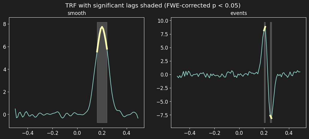
A fitted kernel is only meaningful if it reflects a real stimulus–response relationship rather than noise. pyeeg.stats provides resampling-based inference that works with any solver (unlike the classical tvals_/pvals_, which are only computed on the plain OLS path):

• Permutation test (permutation_test_trf): builds a null distribution by circularly shifting the stimulus (preserving its autocorrelation, breaking the stimulus–response alignment), refitting, and taking the maximum statistic across lags/features/channels — a family-wise error (FWE) correction for free.

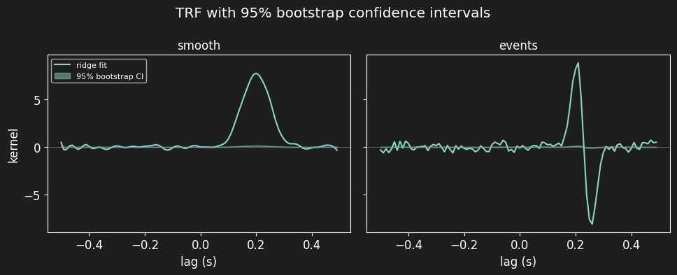
• Bootstrap CI (bootstrap_ci_trf): resamples paired (stimulus, response) blocks and refits, giving a confidence interval per lag.

Both are seeded here for reproducibility. At this data size the permutation test below (200 permutations) and the bootstrap (200 replications) each take a minute or two; pass n_jobs to parallelise.

# Permutation test on the regularised fit (FWE-corrected p-values)
perm = permutation_test_trf(trf_ridge, X, y, n_perm=200, seed=seed)
print(f'min FWE-corrected p: {perm.pvals_corrected.min():.4f}')

reject = perm.pvals_corrected < 0.05
fig = plot_trf_signi(trf_ridge, reject, spatial_colors=False)
fig.suptitle('TRF with significant lags shaded (FWE-corrected p < 0.05)')

min FWE-corrected p: 0.0050

Text(0.5, 0.98, 'TRF with significant lags shaded (FWE-corrected p < 0.05)')

# Bootstrap confidence intervals (paired circular block bootstrap)
boot = bootstrap_ci_trf(trf_ridge, X, y, n_boot=200, seed=seed)
print(f'block size: {boot.block_size_} samples (auto-estimated)')

f, ax = plt.subplots(1, 2, figsize=(10, 4), sharey=True)
for k, name in enumerate(feat_names):
    ax[k].plot(t_kernel, trf_ridge.coef_[:, k, 0], label='ridge fit')
    ax[k].fill_between(t_kernel, boot.ci_low[:, k, 0], boot.ci_high[:, k, 0],
                       color='C0', alpha=.5, label='95% bootstrap CI')
    ax[k].axhline(0, color='gray', lw=0.5)
    ax[k].set_title(name)
    ax[k].set_xlabel('lag (s)')
ax[0].set_ylabel('kernel')
ax[0].legend(fontsize=8)
f.suptitle('TRF with 95% bootstrap confidence intervals')
f.tight_layout()

block size: 208 samples (auto-estimated)

Robust fitting: outliers happen

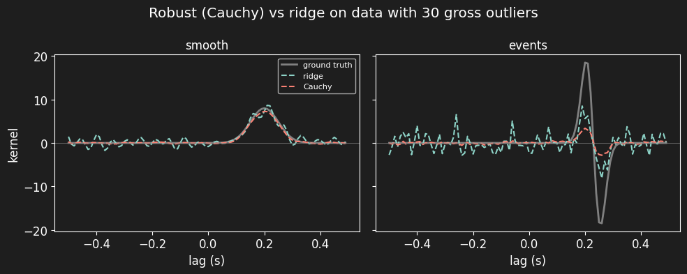
Real data contain artifacts. The default squared-error loss lets a few large outliers dominate the fit. A robust loss — here the Cauchy loss (loss='cauchy', fitted by IRLS) — down-weights large residuals, so gross outliers barely influence the kernel. Below we corrupt 30 samples of y with ±15σ outliers and compare ridge vs Cauchy on the corrupted data.

Notes: robust fits compute no classical t/p-values; robust_sigma sets the Cauchy scale (left to be estimated from the residuals here); robust_solver='least_squares' selects a SciPy reference solver that is ~100x slower (see scripts/examples/solver_showcase.py).

# Corrupt 30 samples of the response with gross outliers (±15 sigma)
y_out = y.copy()
idx = rng.choice(n_samples, 30, replace=False)
y_out[idx] += (rng.choice([-1, 1], 30) * 15 * y.std())[:, None]

trf_ridge_out = TRFEstimator(tmin=tmin, tmax=tmax, srate=fs, alpha=100.).fit(X, y_out)
trf_robust = TRFEstimator(tmin=tmin, tmax=tmax, srate=fs, alpha=100.,
                          loss='cauchy').fit(X, y_out)
print(f'Cauchy fit: converged={trf_robust.robust_converged_}, '
      f'{trf_robust.robust_n_iter_} IRLS iterations, '
      f'scale={np.round(trf_robust.robust_scale_, 3)}')

for name, trf_ in [('ridge ', trf_ridge_out), ('Cauchy', trf_robust)]:
    print(f'{name}: corr(events kernel, truth) = '
          f'{np.corrcoef(trf_.coef_[:, 1, 0], kernel2)[0, 1]:.3f}')

f, ax = plt.subplots(1, 2, figsize=(10, 4), sharey=True)
for k, name in enumerate(feat_names):
    truth = kernel1 if k == 0 else kernel2
    ax[k].plot(t_kernel, truth, color='gray', lw=2, label='ground truth')
    ax[k].plot(t_kernel, trf_ridge_out.coef_[:, k, 0],
              color='C0', ls='--', label='ridge')
    ax[k].plot(t_kernel, trf_robust.coef_[:, k, 0],
              color='C3', ls='--', label='Cauchy')
    ax[k].axhline(0, color='gray', lw=0.5)
    ax[k].set_title(name)
    ax[k].set_xlabel('lag (s)')
ax[0].set_ylabel('kernel')
ax[0].legend(fontsize=8)
f.suptitle('Robust (Cauchy) vs ridge on data with 30 gross outliers')
f.tight_layout()

Cauchy fit: converged=True, 17 IRLS iterations, scale=[8.996]
ridge : corr(events kernel, truth) = 0.693
Cauchy: corr(events kernel, truth) = 0.955

Solvers: same answer, different speed

TRFEstimator solves the (regularised) normal equations with a pluggable solver (pyeeg.solvers). All solvers below solve the same problem — they differ in speed and in what they support:

Solver	Solves	Notes
SVDSolver	ridge (default)	SVD of the normal equations; also a truncated-SVD mode
LSTSQSolver	plain OLS	no regularisation — unstable on ill-conditioned designs
ConjugateGradientSolver	ridge	iterative; attractive for very large problems
IRLSSolver	robust (Cauchy)	IRLS with per-channel convergence
ScipyRobustSolver	robust (Cauchy)	SciPy reference validator, ~100x slower — not timed here

See scripts/examples/solver_showcase.py for a fuller comparison with outliers.

# Timing + accuracy of each solver on the same problem (alpha=100).
# Note the two kernel columns: OLS recovers the well-conditioned event kernel
# but destroys the ill-conditioned smooth one — regularisation is what saves it.
print(f'{"solver":<24}{"fit time":>10}{"corr(smooth)":>14}{"corr(events)":>14}')
for name, solver in [('SVD (ridge)', SVDSolver()),
                     ('LSTSQ (OLS)', LSTSQSolver()),
                     ('CG (ridge)', ConjugateGradientSolver(tol=1e-8)),
                     ('IRLS (Cauchy)', IRLSSolver(max_iter=30))]:
    trf_s = TRFEstimator(tmin=tmin, tmax=tmax, srate=fs, alpha=100., solver=solver)
    t0 = time.perf_counter()
    trf_s.fit(X, y)
    dt = time.perf_counter() - t0
    c1 = np.corrcoef(trf_s.coef_[:, 0, 0], kernel1)[0, 1]
    c2 = np.corrcoef(trf_s.coef_[:, 1, 0], kernel2)[0, 1]
    print(f'{name:<24}{dt * 1000:>8.0f} ms{c1:>14.3f}{c2:>14.3f}')

solver                    fit time  corr(smooth)  corr(events)
SVD (ridge)                  616 ms         0.997         0.988
LSTSQ (OLS)                  964 ms         0.000         0.992
CG (ridge)                   119 ms         0.997         0.988
IRLS (Cauchy)               9961 ms         0.998         0.939

Multi-channel TRFs

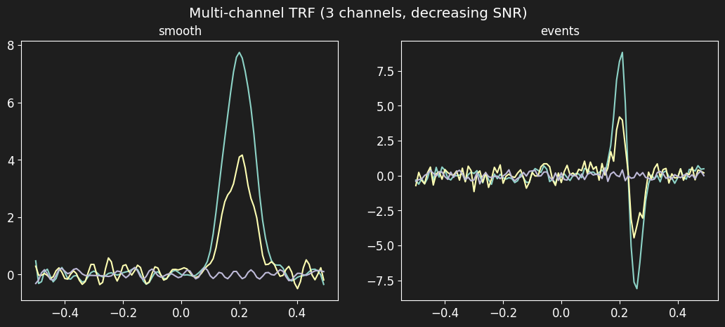
TRF estimation is per channel: fitting y with several columns estimates one kernel per channel (coef_ has shape n_lags x n_feats x n_channels). Multi-channel fits also unlock the group-level statistics in pyeeg.stats (cross_subject_consistency, group_level_test), which need several subjects x channels.

# Three "electrodes" with decreasing SNR
Y = np.column_stack([y[:, 0],                                     # full SNR
                     0.5 * y[:, 0] + 10.0 * rng.standard_normal(n_samples),
                     5.0 * rng.standard_normal(n_samples)])      # noise only
trf_mc = TRFEstimator(tmin=tmin, tmax=tmax, srate=fs, alpha=100.).fit(
    X, Y, feat_names=feat_names)
print('coef_ shape:', trf_mc.coef_.shape, '(n_lags x n_feats x n_channels)')
print('per-channel corr(y, yhat):', np.round(trf_mc.score(X, Y), 3))

fig = trf_mc.plot()  # butterfly plot: one panel per feature, one line per channel
fig.suptitle('Multi-channel TRF (3 channels, decreasing SNR)')

coef_ shape: (100, 2, 3) (n_lags x n_feats x n_channels)
per-channel corr(y, yhat): [0.958 0.767 0.207]

Text(0.5, 0.98, 'Multi-channel TRF (3 channels, decreasing SNR)')

Summary

• A TRF is a linear kernel mapping stimulus to response, estimated over a lag window; here the true kernel peaks at +0.2 s (the response follows the stimulus).

• The smooth, autocorrelated predictor makes the lagged design ill-conditioned, so unregularised OLS blows up; ridge (alpha) fixes it. Select alpha by cross-validation (xfit).

• Use banded regularisation (feature_alphas) to penalise only the features that need it, and quadratic_reg='smoothness' to penalise roughness.

• Judge kernels with resampling inference (permutation_test_trf, bootstrap_ci_trf in pyeeg.stats) — they work with any solver, unlike the classical tvals_/pvals_.

• Real data have outliers: loss='cauchy' fits robustly.

• Estimation is per channel; solvers are pluggable (pyeeg.solvers).

Further reading

• scripts/tutorials/feature_alphas_banded_ridge.ipynb — banded ridge in depth

• scripts/examples/solver_showcase.py — solver comparison with outliers

• scripts/examples/simulated_trf.py — script version of a TRF simulation

• docs/source/stats.rst, docs/source/solvers.rst — API references

• Real data: pyeeg.io loaders (AlignedSpeech, WordLevelFeatures) and the stimulus_features.ipynb tutorial